The UW Liquid Pouring Dataset [full download] focuses on liquids in the context of the pouring activity. It consists of two sub-datasets: A large(er) dataset generated using a liquid simulation engine, and a small(er) dataset collected on a real robot. Each dataset focuses on a cup following a fixed trajectory pouring a clear liquid into a bowl on a table. Each dataset contains sequences of images representing one instance of a pouring action, and includes labels for each pixel in each image. Each sequence varies a different parameter of the activity (e.g., amount of liquid in the cup), and each dataset contains many sequences. The purpose of this dataset is to allow researchers to test their perception and reasoning algorithms for liquids on raw sensory data.
Simulated Dataset
This dataset was generated using a realistic liquid simulator. There are 10,122 pouring sequences, each exactly 15 seconds long (450 frames at 30 fps), for a total of 4,554,900 images.
Data Generation
This dataset was generated using the 3D-modeling application Blender and the library El’Beem for liquid simulation, which is based on the lattice-Boltzmann method for efficient, physically accurate liquid simulations. We separated the data generation process into two steps: simulation and rendering. During simulation, the liquid simulator calculated the trajectory of the surface mesh of the liquid as the cup poured the liquid into the bowl. We varied 4 variables during simulation: the type of cup (cup, bottle, mug), the type of bowl (bowl, dog dish, fruit bowl), the initial amount of liquid (30% full, 60% full, 90% full), and the pouring trajectory (slow, fast, partial), for a total of 81 simulations. Each simulation lasts exactly 15 seconds for a total of 450 frames (30 frames per second).
Next we rendered each simulation. We separated simulation from rendering because it allows us to vary other variables that don’t affect the trajectory of the liquid mesh (e.g., camera viewpoint), which provides a significant speedup as liquid simulation is much more computationally intensive than rendering. In order to approximate realistic reflections, we mapped a 3D photo sphere image taken in our lab to the inside of a sphere, which we placed in the scene surrounding all the objects. To prevent overfitting to a static background, we also added a plane in the image in front of the camera and behind the objects that plays a video of activity in our lab that approximately matches with that location in the background sphere. This image shows the setup:
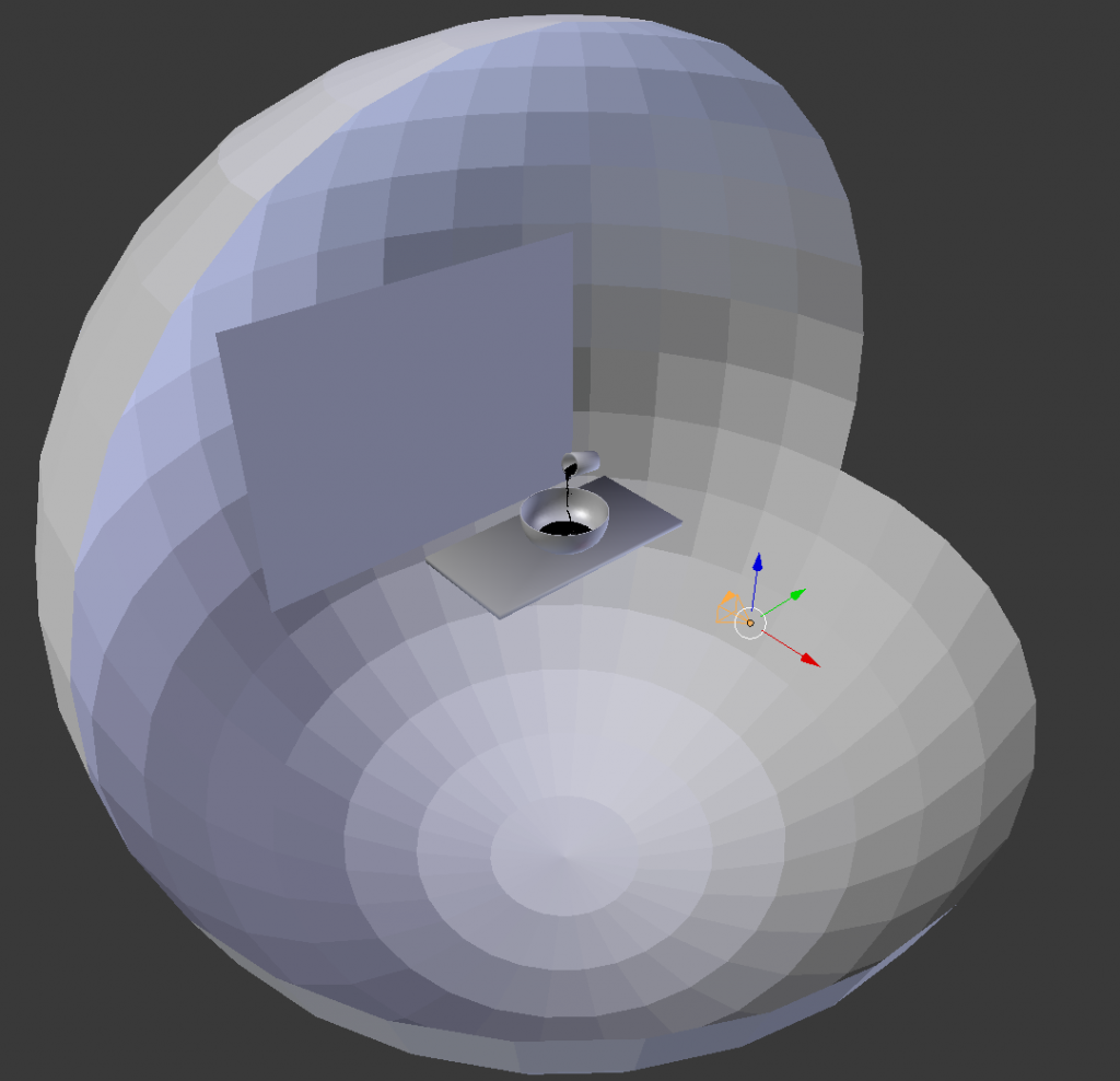
The objects are shown above textureless for clarity. The sphere surrounding all the objects has been cut away to allow viewing of the objects inside. The orange shape represents the camera’s viewpoint, and the flat plane across the table from it is the plane on which the video sequence is rendered. Note that this plane is sized to exactly fill the camera’s view frustum. The background sphere is not directly visible by the camera and is used primarily to compute realistic reflections.
The liquid was always rendered as 100\% transparent, with only reflections, refractions, and specularities differentiating it from the background. For each simulation, we varied 6 variables: camera viewpoint (48 preset viewpoints), background video (8 videos), cup and bowl textures (6 textures each), liquid reflectivity (normal, none), and liquid index-of-refraction (air-like, low-water, normal-water). The 48 camera viewpoints were generated by varying the camera elevation (level with the table and looking down at a 45 degree angle), camera distance (close, medium, and far), and the camera azimuth (the 8 points of the compass). We also generated negative examples without liquid. In total, this yields 165,888 possible renders for each simulation. It is infeasible to render them all, so we randomly sampled variable values to render.
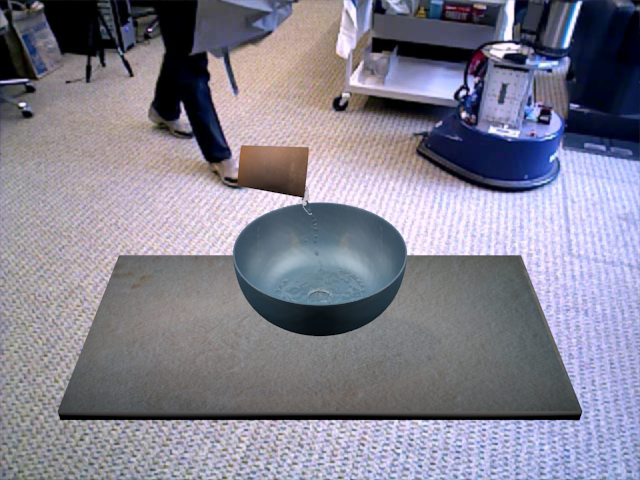
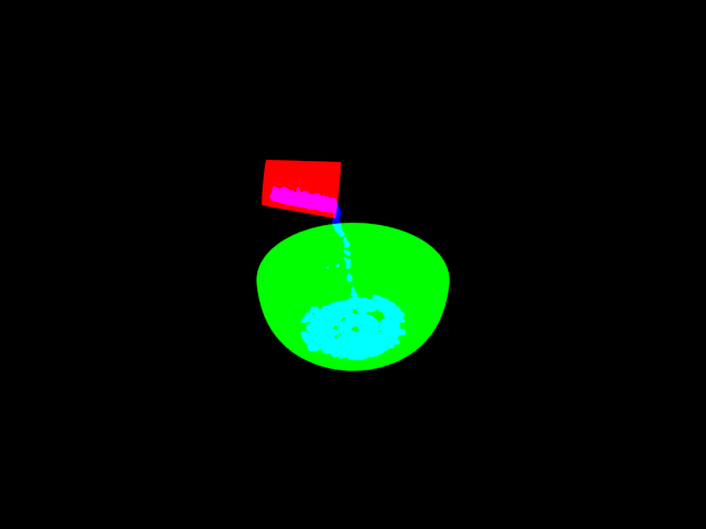
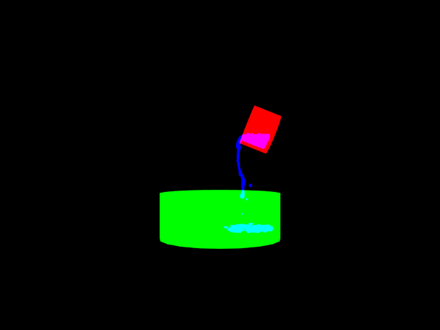
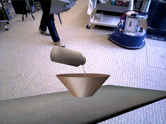
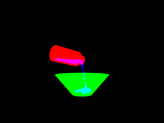
Example Data
|
|
|
|
 |
 |
|
 |
 |
|
 |
 |
Data Layout
The layout for the simulated dataset is as follows (… indicates multiple files):
- Rendered Images
- … Simulation – One folder for each of the 81 simulations.
- … Render – One folder for each render of each simulation, i.e., each sequence.
- … dataN.png – The rendered color image for each frame, where N indicates the frame.
- … ground_truthN.png – The pixel-wise ground truth for each frame, where N indicates the frame. The red channel indicates pixels that belong to the cup; the green channel indicates pixels that belong to the bowl; the blue channel indicates pixels that are liquid; and the alpha channel indicates which is visible at each pixel (0 for red, 128 for green, 255 for blue. Note that if all three color channels are 0 at any pixel, the alpha value is undefined).
- args*.txt* – Files of this format indicate the variable values used to create this render
- bounding_boxes_all.txt – Each line indicates the bounding box, in pixels, of each of the color channels of the ground truth images for each frame, i.e., a bounding box for each object in each image. Note that each line is directly interpretable by the python interpretor.
- bounding_boxes_visible.txt – Similar to above except it only includes pixels of each object that are visible in each frame (e.g., if the cup is partially occluded in a frame, it will only draw a bounding box around the visible portion).
- data.avi – (optional) A video comprised of all the dataN.png images.
- lop_loc.csv – A comma-separated file that indicates for each frame, the XY location in pixels of the lip of the cup.
- … Render – One folder for each render of each simulation, i.e., each sequence.
- … Simulation – One folder for each of the 81 simulations.
- Simulation Files (separated from the rendered files for faster access)
- … Simulation – One folder for each of the 81 simulations.
- args*.txt* – Files of this format indicate the variable values used to create this simulation
- bowl_volume.csv – A comma-separated file that indicates the volume of liquid in the bowl (in m3) at each frame of the simulation.
- scene.blend – The Blender file for this simulation.
- bake_files – Folder containing the Blender files generated by the liquid simulation.
- … Simulation – One folder for each of the 81 simulations.
Download page for the LPD dataset
Real Robot Dataset
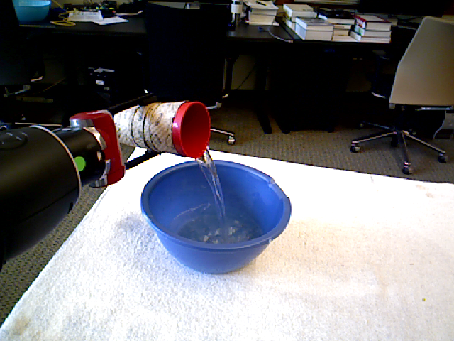
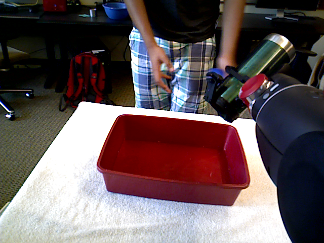
This dataset was generated using a Baxter Research Robot. We recorded 648 pouring sequences with the robot, each lasting approximately 25 seconds.
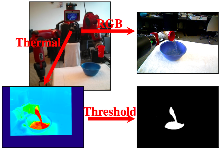
Data Generation
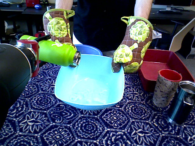
The data was collected on a Baxter Research Robot with an Asus Xtion Pro and an Infrared Cameras Inc. 8640P thermographic camera mounted to the robot’s chest, just below its display screen. During each pouring sequence, the robot’s arm was fixed with a cup in the gripper above the bowl, which was placed on the table in front of it. The robot rotated only its last joint (i.e., its wrist), and it followed a fixed trajectory. During each pour, the robot recorded images from its RGB, depth, and thermographic sensors, as well as its joints states. The thermographic images were then normalized across the entire sequence and thresholded to acquire the ground truth labelling.
We varied the following variables across different sequences:
- Arm [right, left]
- Cup [cup, bottle, mug]
- Bowl [bowl, fruit bowl, pan]
- Water Amount [empty, 30%, 60%, 90%]
- Pouring Trajectory [partial, hold, dump]
- Movement [minimal, moderate, high]
We collected data for every permutation of these variables, resulting in 648 sequences collected on the real robot.
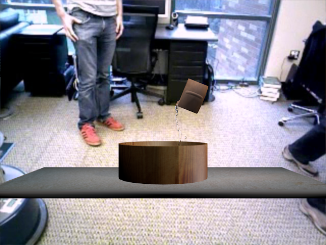
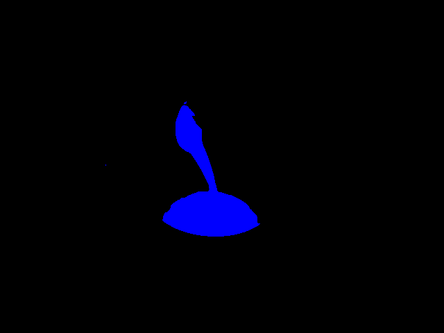
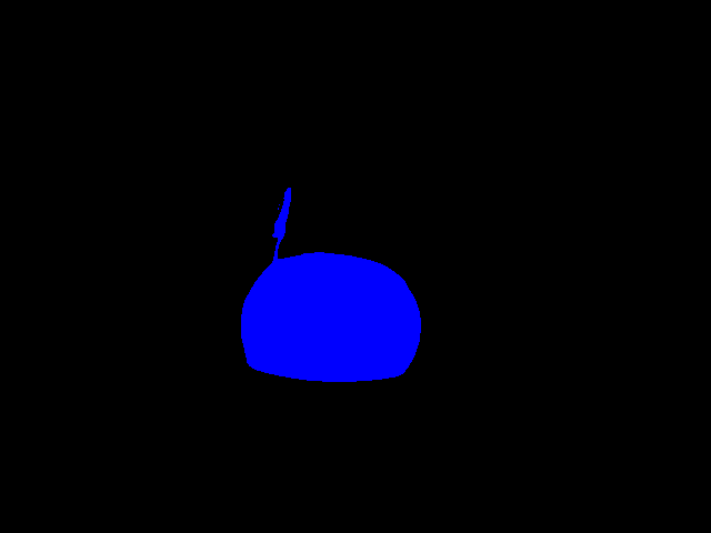
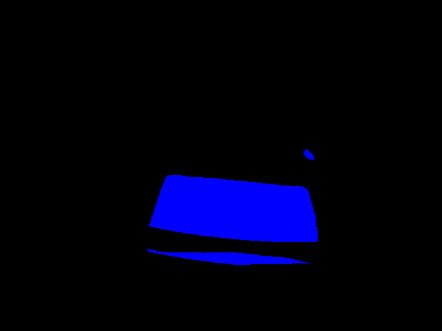
Example Data
|
|
|
|
 |
 |
|
 |
 |
|
 |
 |
Data Layout
The layout for the real robot dataset is as follows (… indicates multiple files):
- Images – The pre-processed images collected from each sequence
- … Sequence – One folder for each of the 648 sequences. Note: These files have the same format as for the simulated dataset for compatibility reasons, though some of that format is superfluous.
- … dataN.png – The color image for each frame, where N indicates the frame.
- … ground_truthN.png – The pixel-wise ground truth for each frame, where N indicates the frame. The blue channel indicates pixels that are liquid.
- args*.txt* – Files of this format indicate the variable values used to create this sequence.
- bounding_boxes_all.txt – Each line indicates the bounding box, in pixels, of each of the color channels of the ground truth images for each frame. Note that each line is directly interpretable by the python interpretor.
- bounding_boxes_visible.txt – Identical to above. This is kept for compatibility reasons.
- … Sequence – One folder for each of the 648 sequences. Note: These files have the same format as for the simulated dataset for compatibility reasons, though some of that format is superfluous.
- Raw Data – The raw, unprocessed data collected for each sequence. This is kept separate from the images for ease of access.
- … Sequence – One folder for each of the 648 sequences.
- args*.txt* – Files of this format indicate the variable values used to create this sequence.
- data.bag – ROS bag-file that contains all the raw data. It contains data from the following topics:
- /camera/rgb/image_color – Color images collected from the Asus Xtion Pro.
- /camera/depth_registered/image_raw – Depth images collected from the Asus Xtion Pro. Each pixel is an unsigned short that gives the depth at that point in millimeters.
- /ici/ir_camera/image – Thermal images collected from the ICI 8640P thermographic camera. Each pixel is an unsigned short and its value corresponds to the raw IR sensor reading, which is related to the temperature at that pixel.
- /ici/ir_camera/calibration – A string message that represents the affine transformation between the color image pixel space and the thermal image. Given the 3×3 transformation matrix M and a point p=<x,y,1> in color pixel space, p’=p*M is that point in thermal pixel space. Note that this transformation is only valid for a fixed distance from the camera. We calibrated this transform to be the depth of the robot’s gripper during all sequences. The first line of the string message is the resolution of the color image, and the following 3 lines are the matrix M.
- /robot/joint_states – The state of the robots joints across the sequence.
- … Sequence – One folder for each of the 648 sequences.